SP2LNOB Methodology

The Social Protection to Leave No One Behind (SP2LNOB) App combines a machine learning algorithm with a linear micro simulation model with Household Income and Expenditure Surveys (HIES) from Cambodia and the Maldives as underlying survey data. The App follows a two-pronged methodology. First, it models and identifies population groups in both countries with different access to basic opportunities such as access to the internet. In doing so, it disaggregates the national average access rate. In the next step, the App allows users to distribute cash transfers to eligible recipients in line with selected social protection schemes. In this step, the App quantifies and visualizes improvements, if any, in access to opportunities following the cash transfer among pre-identified population groups in the first step. Following these two steps, the App connects social protection as a policy tool to outcomes associated with leaving no one behind in inclusive and sustainable development.

The first step leverages the Classification and Regression Tree (CART) methodology, which is a type of supervised machine learning algorithm that predicts a given outcome (i.e. access to the internet) based on a predefined set of circumstances (i.e. age, sex, location education, income and disability status), using a decision tree structure. More specifically, the App relies on binary regression trees, or LNOB trees for short, using analysis of variance as its splitting criterion. LNOB trees provide an intuitive visualization of mutually exclusive population groups with distinct outcomes. Moving beyond simple disaggregation in the form of cross-tabulations for a given circumstance separately, the CART methodology includes all circumstances simultaneously and identifies their intersections (e.g. older men living in poorer and rural households). For more details, please see the methodology section of the ESCAP LNOB Platform.

The algorithm repeatedly splits the data based on selected circumstances. Each split creates two non-overlapping groups, with each group representing a node in the tree. The goal is to find splits that minimize the variance of the selected outcome within each group. At each node, the algorithm selects the circumstance and threshold that provides the best split in the outcome variable according to a particular loss function. This process continues until the tree is fully grown (i.e. until the data cannot be split any further across the set of selected circumstances), or until one of the specified stopping criteria is met (e.g. complexity parameter^[a] and minimum split size^[b]).

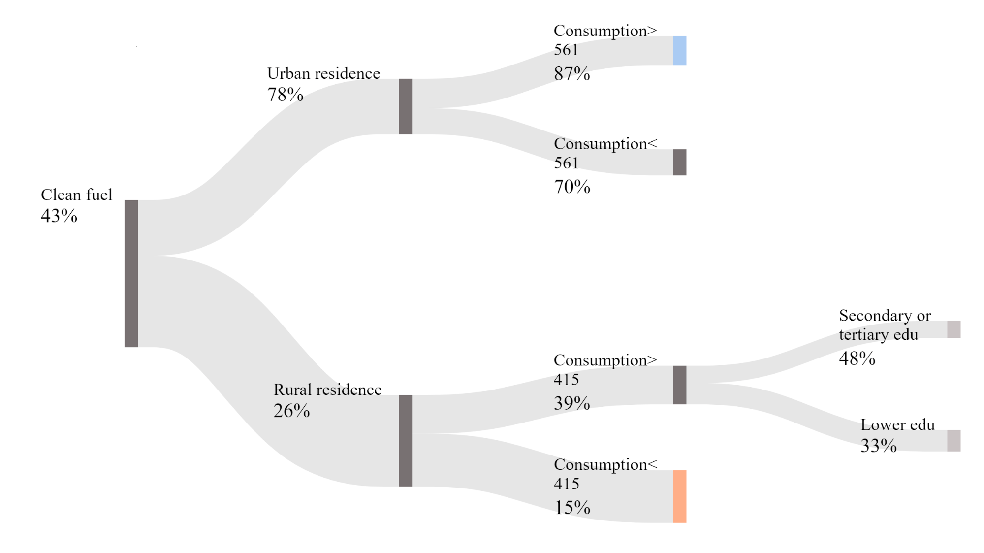
Figure 1 below presents one such tree, which disaggregates access to clean fuels for cooking in Cambodia based on the 2019-2020 Cambodia Socioeconomic Survey. The tree starts from a root note that represents the national average which in this case indicates that 43 per cent of households in Cambodia had access to clean fuel. The algorithm finds that different households have different access rates with residence, monthly expenditure per capita and education level of household head intersecting in identifying these household groups. For instance, access is considerably lower among rural households with a household expenditure of less than 415,000 Cambodian riel. Only 15 per cent of those households enjoy access to clean fuel. Since they have the lowest average group access rate, they represent the furthest behind group denoted in orange. Note that some households in the furthest behind group still have access to clean fuels. However, 85 per cent of the furthest behind group (i.e. 100 per cent – 15 per cent) do not have access to clean fuels. There is no other group identified in the tree with a lower average access to clean fuels. On the other hand, urban households who have a monthly household expenditure per capita of more than 561,000 Cambodian riels have an access rate of 84 per cent. This group represents the furthest ahead group, denoted in blue, in Cambodia as there is no other group with an average access rate that is higher than 84 per cent. Among this group, a small share of households (i.e. about 16 per cent of households) do not have access to clean fuels. Hence, the furthest ahead group does not have universal access either. In addition to the furthest ahead and furthest behind groups, the LNOB tree also identifies three other groups in terminal nodes. Hence, in disaggregating this indicator, the algorithm identified five groups. A weighted average of their access rates reverts back to the national average of 43 per cent.

Figure 1: Regression tree estimating differences in access to clean fuel, low complexity

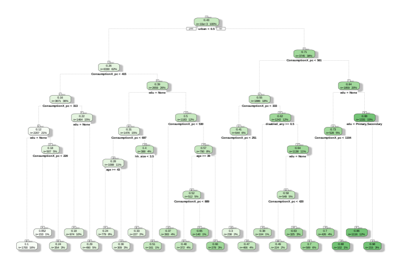
The number of terminal nodes in Figure 1 depend fundamentally on the specified stopping criteria parameters. For instance, Figure 2 also disaggregates access to clean fuels in Cambodia using the same set of circumstances, but it does so using a lower complexity parameter. The visualization is different than Figure 1 because the former is based on ESCAP LNOB Platform visual styling while the latter is a raw output from the statistical software programme R. The complexity parameter restricts the amount of tree nodes by only allowing splits that improve the R-squared coefficient by at least the value of the parameter. In the R package rpart, the complexity parameter is scaled from 0 to 1, where cp = 1 will always result in a tree with zero splits. Consequently, the tree in Figure 2 that was estimated using a lower complexity parameter consists of 25 terminal nodes, a marked contrast to the tree in Figure 1, which has only 5. When selecting an appropriate complexity parameter, it is crucial to strike a balance between bias and variance. A smaller parameter may lead to a more intricate tree, potentially capturing finer nuances, but also risks overfitting to noise in the data, while a larger parameter may yield a simpler, more interpretable tree but might miss important patterns.

Figure ^[c]2: Regression tree estimating differences in access to clean fuel, high complexity

The SP2LNOB App uses the output from the LNOB tree to benchmark current inequality or differences in access to clean fuels between population groups in Cambodia. Concretely, the predicted mean access to a given indicator is assigned to each terminal node in the tree.

In the second step, the App simulates the impact of cash transfer programs in line with ESCAP SPOT Simulator. Specifically, it increases household expenditure among eligible households by a specific amount selected by the user. For more details, please see the methodology of the ESCAP SPOT Simulator. This increase in household expenditure may move some households from one terminal node into another.  Since higher household expenditure is generally associated with higher levels of access, these cash disbursements generally lead to an improvement in access rates. This may not always be the case, however. If household expenditure is not featured as a variable in the LNOB tree, then the groups identified in terminal nodes are not based on household expenditure thresholds. Therefore, receiving cash transfer will not prompt a move to a higher access group. This is because, in the absence of expenditure variable, higher access to opportunities by other groups is driven by other circumstances such as age, location or education.

Figures 3 to 5 presents a simple example focusing on access to internet in the Maldives based on the 2019 Household and Income Expenditure Survey. Figure 3 presents the LNOB tree for access to internet at household level. The root note shows that at on average 68 per cent of households in the Maldives had at least one member with access to the internet. In other words, 32 per cent of households did not have any member with access to the internet.

The disaggregation model includes location of household, monthly per capita consumption expenditure, age, sex, education of the household head and whether there are any persons with disability in the household.  The LNOB tree below presents the results of disaggregation based on the machine learning algorithm checking for a large set of combinations behind the scenes. The algorithm finds that location is the most important variable as it can explain the variation much better than other circumstances. Hence, the first split is location. While 84 per cent of households living in Male have at least one household member with access to the internet, this figure drops to 54 per cent in the atolls outside the capital. Among households living outside Male, monthly expenditure per capita can explain more variation relative to other circumstances such as age and sex of household head or disability status among household members. Those with less than MVR 2019 have the lowest access rate at 35 per cent, while 57 per cent of relatively richer households (still living outside Male) have access. The algorithm finds more variation among the latter group or the relatively richer households living outside Male. Specifically, access to the internet is lower among households with at least one person with a disability and living outside Male with a monthly expenditure per capita of MVR 2019 and above. In this part of the tree, lowest access rate is among relatively poorer households, among whom 35 per cent report access while 65 per cent lacks access. They are the furthest behind group as there is no other group identified with lower access rate.

Figure ^[d]3: LNOB tree estimating differences in access to internet in Maldives (2019)

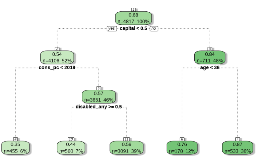
The LNOB tree identifies variation among households living in Male, as well. The age of household heads makes a difference. Households headed by individuals less than 36 have slightly lower access to internet than households headed by individuals 36 and above. The furthest ahead group is represented by households living in Male and headed by an individual over the age of 36. Access to internet is the highest in this group with 87 per cent of such households reporting that at least one member has access to the internet. Notably, in this furthest group not all households have access to the internet. In fact, 13 per cent of households living in Male with a household head aged 36 and above report no access to the internet.

Consequently, the LNOB tree started from the national average of 68 per cent and then identified 5 groups in its terminal nodes. It started with a sample of 4,817 households and split these households into distinct groups across five terminal nodes with significantly different access rates. A weighted average of access to the internet across these five groups will yield the national average.  At this point, the first step of the SP2LNOB is completed.

In the second step, the App allows users to extend social protection schemes in the form of cash transfers. The online version of the App presents three key schemes, namely (i) child benefits for all children under 18, (ii) old age pensions for all older persons aged 65 and above and (iii) disability benefits for all persons with severe disabilities. Users have several options. They can choose the benefit amount associated with each scheme. They can also choose one scheme or a combination of schemes with different benefit amounts. The default option in the App is to distribute all three schemes based on global average benefit amounts universally to all eligible households. Users also have an option to provide means-tested schemes whereby an additional eligibility is introduced based on proxy means testing. In this option, they can distribute the cash transfer to poorest households only. In doing so however, they should bear in mind that poor households are identified based on their assets and not their monthly expenditure. This often leads to large exclusion and inclusion errors.

In the case of default universal schemes, child benefits are distributed per children to all households with children aged 0 to 17 at 4 per cent of GDP per capita per annum. Households with no children in this age category do not receive any benefits. Similarly, 14 per cent and 16 per cent of GDP per capita per annum is distributed to each older person and person with severe disability in the household.  Depending on the choices of the user, a household may receive multiple benefits thanks to the eligibility of its household members. Users can modify benefit amounts in line with their preferences. Note that the offline version of the App allows users to introduce other schemes as they deem fit to mimic existing schemes in their countries.

In the App, the first objective of this step is to identify which households are eligible and how much money they should receive in local currency. The underlying data allows this selection with ease thanks to the availability of associated variables such as age and disability status. Since the LNOB tree is disaggregated with total monthly household expenditure per capita, the App in this step injects cash transfers in per capita and per month frequency. Once the cash transfer is distributed, the next step is guided by the terminal nodes identified in the LNOB tree (Figure 3) and the size of the total benefit received by households. If monthly expenditure per capita is displayed in the LNOB tree with a specific monthly household expenditure per capita threshold, then it is possible that the selected social protection schemes push recipient households beyond the predefined expenditure thresholds.

In this static simulation model, the only change that households experience is an increase (if any) in their total household monthly expenditure per capita thanks to social protection. None of the other characteristics change. By construction and model assumptions elaborated later below, households cannot change other circumstances such as their location following a cash transfer. The age, sex or disability status of the household head or household member cannot change after cash transfers.

Figure 4 below presents the findings of the App after the distribution cash transfers. Specifically, it displays the distribution of households in terms of their access to internet before and after cash transfer. The five groups of households stacked up on either side of the diagram correspond to the five terminal nodes of the LNOB tree in Figure 3. In its center, the diagram shows transitions among groups due to increased monthly expenditure per capita.

Figure 4: Distribution of population groups before and after cash transfer

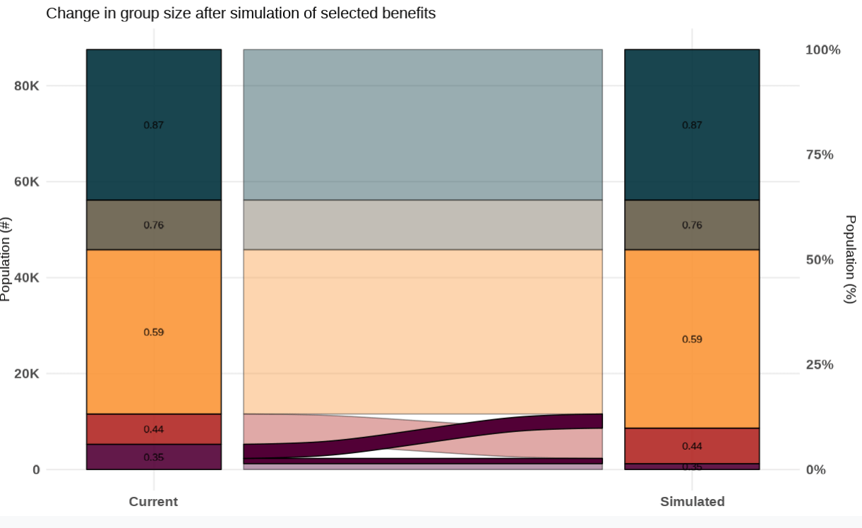
As indicated earlier, a transition is expected if and only if household expenditure is featured in the LNOB tree and cash transfers push upward from their current group to a higher expenditure group. No movement can be observed otherwise. For instance, consider the households living in the capital, Male, who are headed by individuals aged 36 and above. In Figure 4, they are represented by the dark green box on the very top of the two columns on either side of the diagram. Recall that among these households 87 per cent had access to the internet. Right below them, households still living in Male but headed by individuals under 36 years of age are presented in lighter gray. Before and after the cash transfer, these groups stay identical with no transitions from one to the other. This is because household expenditures did not create a split in Male. Rather, age of household head did. Since the head of household cannot change his or her age based on the cash transfer, the two groups remain the same. Note that some of these “higher access to internet” households may have received cash transfers selected by the user.

The situation is more interesting for households living outside Male where household expenditure matters. Recall that the furthest behind group is represented by households living outside Male with a monthly total household expenditure per capita that is less than MVR 2019. In the diagram above, they are at the very bottom of the stacked column in purple color. Among them 35 per cent reported that at least one household member had access to the internet. The next group in orange color represents households living outside Male with at least one person with disability and total monthly household expenditure per capita equal to or higher than MVR 2019. Among these households 44 per cent reported access to the internet. Finally, the third group represents households who are living outside Male with no persons with disability in the households and total monthly household expenditure per capita equal to or higher than MVR 2019.

Figure 4 shows that after the cash transfer, some but not all of the furthest behind group transitioned to two “higher access” groups. The total benefits received helped these households move beyond the MVR 2019 threshold. These two upward transitions are represented by the dark shaded purple lines in the middle of the diagram.

1. The first transition is represented by a relatively thicker dark purple line. It includes households who had less than MVR 2019 and no person with disability before the cash transfer. After the cash transfer, they passed the expenditure threshold and moved to the relatively richer group of households with no persons with disabilities.

2. The second transition is captured by a thinner dark purple line which shows that a smaller group of furthest behind households who also had less than MVR 2019 but they had at least one person with disability before the cash transfer. After the cash transfer, they passed the expenditure threshold, but the simulation placed them in the “44% access group” as opposed to the “59% access” group. This is because moving to “59% access” group consists of households above the expenditure threshold and with no persons with disabilities.

There is no other upward movement originating from the furthest behind group. The unshaded purple line represents households who did not move anywhere and remained as furthest behind. Perhaps, they did not have any eligible household members, so they did not receive any cash transfers. Alternatively, they may have received some cash transfers, but it was not large enough to help them move beyond the MVR 2019 expenditure threshold.  A larger cash transfer may move some or all of them to the next two groups. The user can experiment with different benefit amounts and simulate the results.

Note that the three groups at the bottom of the stacked columns are living outside Male. Irrespective of the size of the cash transfer or the importance of household expenditure in affecting access to internet, they cannot move to the top two groups. This is because the top two groups live in Male. Cash transfers cannot prompt households change their location by the assumption of the model which is a reasonable underlying assumption. While cash transfers can expand disposable income and thereby increase expenditures, it is unlikely that they affect more complex decisions like migration.

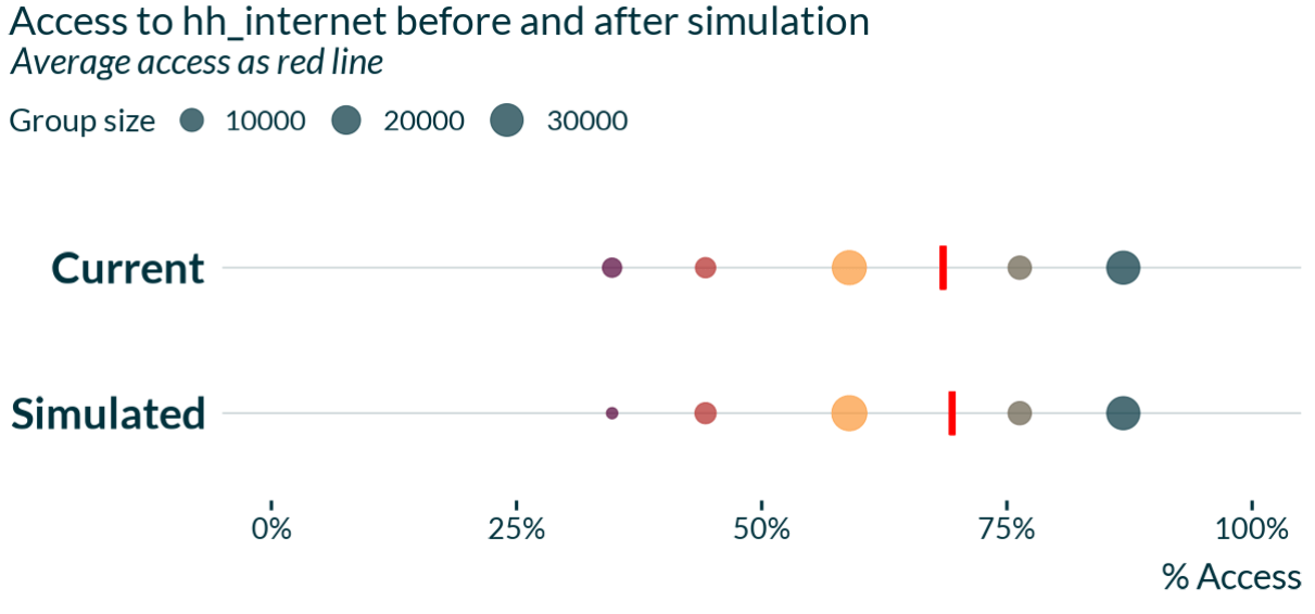
Figure 5 below provides a summary of the groups before and after the cash transfers. The five groups are represented as five dots on a number line which represents access to the internet. The five groups are the same as those shown in Figures 3 and Figure 4. The main change before and after cash transfers is the size of some of the groups in line with Figure 4. Recall that the dark purple dot under current situation is much larger than the same dot under the simulated scenario. After the cash transfer, some furthest behind moved upward and the size of the furthest behind shrank. Figure 4 above showed where those two groups from the original furthest behind moved next. Thanks to this shift, the size of the orange and yellow dots increased slightly under the simulated scenario. Notice that no change is visible in the lighter and darker greener dots. Finally, the red line in Figure 5 represents the national average access to internet among households. While it was 68 per cent before the cash transfer, it increased to XX ^[e]per cent after the cash transfer. This was driven by the two upward movements out of furthest behind group. Now that there are more people in “higher access” groups, the weighted national average has slightly increased.

It is important to emphasize that this modeling strategy assumes that, following the distribution of cash transfers, eligible households will instantaneously obtain the same access rate to basic social resources (or prevalence of barriers) as the new group to which they are assigned to. In practice, however, there may be multiple reasons for differences in access, as well as time lags in outcome changes. Therefore, the results of these simulations should be understood as hypothetical scenarios, rather than as causal estimates of the effect of cash transfer programs on the outcomes.

There are several limitations and assumptions of this methodological approach that should be borne in mind when interpreting the results of the SP2LNOB APP.

First, the LNOB trees aim to gauge the distribution of access to a specific outcome among observable characteristics. However, there are likely additional unobserved factors that also influence access rates. Notably, there may be omitted variables that simultaneously contribute to both low access levels for a particular outcome and low household income, consumption, or expenditure. In such scenarios, the underlying model may indicate that enhancing household income through cash transfers would enhance access rates, even though the true reason for the lack of access is another omitted variable. Take, for instance, this example: households in a specific, poor region lack access to the electricity grid. Because region is not included as a circumstance in the LNOB tree while household income is, the model might suggest that boosting these households’ income through a specific social protection scheme would elevate their electricity access, despite the root cause of the access deficiency being the specific region in which these households are situated.

Another limitation concerns the estimates of inequality in access, since these estimates depend in part on the number of terminal nodes that are considered. A model that relies on a very small tree with only one terminal node will have no inequality in access, since everyone in the sample gets assigned the same level of average access. As the number of terminal nodes increases, the inequality parameters also increase. This is because as the tree grows potentially due to the inclusion of more circumstances, it captures more groups with difference access rates in its terminal nodes. For this reason, it is best to compare changes between the current and simulated results for the same tree, rather than comparing results between trees with different parameter specifications.

A third limitation concerns the allocation of cash transfer itself. The App assumes that cash transfers are assigned perfectly and instantly to all eligible households across the country. Furthermore, the App also assumes that 100 per cent of the cash transfers are translated into an increase in household consumption. Hence, there are no savings. In practice, however, the allocation of cash transfers would not happen instantaneously, and would arguably not lead to a linear increase in expenditure.

It is very important to keep these assumptions and limitations in mind when interpreting the results of the SP2LNOB App. The simulated results should be understood as hypothetical scenarios rather than as causal estimates of the effect of cash transfer programs on access to opportunities. To robustly assess the effect of social protection schemes on access rates, it is necessary to conduct a robust experimental design, such as through a randomized control trial.